Pricing for water conservation with cost recovery
[1] Variable unit pricing provides incentives for conservation, similar to increasing block rates, while covering system costs. For supply‐limited situations and planning contexts, it is also shown to provide for cost recovery with supply limits and capacity constraints. This paper presents two applications of pricing with supply constraints: (1) an application for Amman, Jordan, showing that VUP satisfying a supply limit can avoid more costly capacity expansion and (2) an example of seasonal pricing for Boulder, Colorado, as an alternative to water restrictions. These two cases also exhibit two methods for generating data needs: (1) a “full information approach” with specified demand and cost functions and (2) “iterative pricing” that uses a previous year’s cost and consumption data to set future pricing.
1. Introduction
[2] In many water supply systems, water rates are being redesigned in light of recent droughts that focus attention on conservation needs. The use of increasing block rates (IBR) has become prominent for conservation purposes, and has been recommended by the U.S. EPA for this purpose [Duke and Montoya, 1993] (see also http://www.epa.gov/waterinfrastructure/pricing/About.htm). However, IBR has shortcomings: first, definition of block sizes and associated prices is arbitrary; second, there can be problems with respect to cost recovery as consumers cut back on water use. Utilities have faced revenue losses of up to 14% because of demand reductions [Bishop and Weber, 2001].
[3] Variable unit pricing (VUP) was developed to cover costs while satisfying economic efficiency [Loehman, 2004]. Here, its use is extended for satisfying a supply limit or meeting a seasonal capacity constraint while covering cost and satisfying economic efficiency. VUP can also achieve cost recovery for long‐term investments for sustainability by including bond payments among the fixed costs to be covered each period (E. T. Loehman, Sustaining groundwater through social investment, pricing, and public participation, unpublished manuscript, 2008, available from the author).
[4] An intended context for variable unit pricing is water demand management and planning, when water utilities and others concerned with water management engage in determining the desired level of supply, such as a supply limit relative to expansion needs and drought. In this context, in addition to covering costs, variable unit pricing can provide incentives for demand to meet the desired supply. (See section 7 for further discussion.)
[5] Criteria for utility pricing include fairness as well as economic efficiency and cost recovery [Brown and Sibley, 1986]. Economists support the criterion of economic efficiency (total net benefit maximization), because otherwise a change in allocation or supply could be made that would benefit at least some consumers of a water system without hurting others. Zajac [1979, ] has discussed the importance of fairness for utility pricing. Objectivity is a related social criterion: rates should be determined by well‐specified rules not dependent on personal identity. If rates are perceived to be unfair or not objective, the rate setting process can become politicized and open to rent seeking [Hall and Hanemann, 1996].
[6] VUP satisfies a fairness property in that the total water bill for each consumer is a proportion of total cost according to the share of water consumption. VUP satisfies objectivity because pricing parameters are specified by formula on the basis of cost properties and use levels. In contrast, IBR has no formula for determining pricing parameters, so that cost recovery can only be satisfied through trial and error. For example, if IBR has three rate blocks, there are two “jump points” and three price levels to determine for the rate schedule, in total five parameters to determine for each consumer type. The last block is sometimes set equal to long‐run marginal cost for economic efficiency reasons; even so, there will still be four parameters to determine for each consumer type.
[7] Consumer understanding of billing procedures is another important pricing issue. Boland [2000] has suggested that for consumer understanding, a simpler rate structure than IBR would be desirable. With IBR, a consumer does not have an easy task to determine the total bill; charges must be added up over ranges of consumption. Because of rate complexity, the effects of IBR on consumer demand are controversial, e.g., whether consumers consider marginal or average prices when determining water consumption [Shin, 1985; Nieswiadomy and Molina, 1991].
[8] In contrast, VUP provides a relatively simple rate structure based on a per unit charge: all units consumed are charged at the same rate. The total bill is simply the unit price, specified for the level of total consumption, times total consumption. Table 1 illustrates the unit price schedule given by ranges of use for a case of increasing costs.
Table 1. Illustration of Variable Unit Pricing Charge Schedule
a
| Water Use |
Unit Price |
Total Bill |
| 500 |
$0.0383 |
$16.67 |
| 1000 |
$0.0433 |
$43.30 |
| 3000 |
$0.0633 |
$189.90 |
| 5000 |
$0.0833 |
$416.50 |
[9] The unit price is specified to vary linearly with water consumption. Figure 1 illustrates the unit charge schedule for VUP when the unit charge is increasing (it can also be decreasing, depending on cost properties). Increasing unit price provides a conservation incentive similar to IBR in that greater consumption will entail a higher unit price and hence a higher total bill.
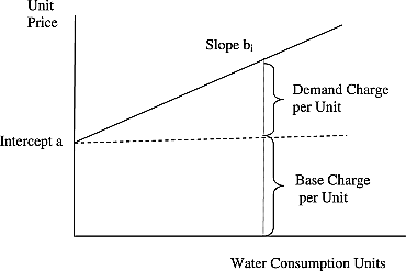
Figure 1
Illustration of variable unit pricing.
[10] The terms “base” and “demand” charges are familiar for water pricing. The VUP charge per unit is the base charge plus the demand charge per unit. In Figure 1, the base charge per unit is the intercept. The demand charge per unit is the slope times the consumption level.
[11] The following sections derive slope and intercept formulas for unconstrained and constrained supply situations. Readers who do not wish to pursue details are invited to skip these sections. The paradigm for parameter determination is a generalization of the first theorem of welfare economics [Bohm, 1976] to nonlinear (nonconstant) pricing; for more discussion, see [Loehman, 2004]. For a water economy with variable unit prices, the pricing paradigm is as follows.
[12] 1. Define a social problem expressing the desired outcome (economic efficiency (EE)) with constraints (supply, capacity, etc.) as appropriate.
[13] 2. Define a water supply demand equilibrium on the basis of variable unit pricing for consumers and the water utility that satisfies the EE problem.
[14] 3. Determine slope and intercept parameters for variable unit pricing to satisfy EE with cost recovery.
[15] After parameter formula development, two case studies for supply limits and capacity constraints also highlight two types of data/computation methods: “full information” utilizing both cost and demand functions, and “iterative pricing” using data from a previous year to develop pricing for a subsequent period. The theoretical properties of efficiency and cost recovery may only be approximately satisfied in real applications of pricing formulas.
[16] Below, the derivation of slope and intercept formulas is presented for individual consumers. However, utilities more conveniently provide rates by consumer type, such as households, commercial and industrial, etc. Therefore, Appendix Aconsiders parameter formulas by consumer types, indicating that theoretical efficiency is only approximately satisfied when pricing is determined by consumer types. For VUP by consumer type, the average user of a given type is charged the average unit price, equal to average cost; use levels greater than average are charged more than average cost, and the converse holds for use levels less than average use.
[17] In the derivation of parameter formulas, wi represents water use by consumer i and pi represents the unit price for this water use: pi = a + biwi. The corresponding total bill or charge schedule is unit price times total consumption: Ri(wi) = (a + biwi)wi. The intercept (a) and slope parameters (bi) are determined by the two requirements of economic efficiency and cost recovery, as shown below. The same intercept applies for all consumers.
[18] Pricing must cover joint cost C(Σwi) of total water production Σwi. Joint costs include raw water costs, drinking water treatment costs, and administrative costs. Cost may also include a fee or return to entrepreneurship, when there is a private supplier.
[19] Utility situations usually also have separable costs, e.g., larger pipes for larger water consumers and pumping stations for more isolated locations. With separable costs, total costs can be covered without affecting efficiency conditions if nonvolumetric separable charges for individual consumers are simply added to volumetric charges.
2.1. Economic Efficiency (EE) for Water Supply
[20] For economic efficiency [Bohm, 1976], supply and allocation should maximize total community net welfare, here expressed in dollar terms. Given benefit functions Bi(wi) for water consumers with use levels wi and the joint cost function C(Σiwi) for total supply Σiwi, the efficient allocation, here without supply constraints, should maximize total net benefits:
[21] First‐order necessary conditions for efficiency are that the marginal benefit (MB) (derivative of benefit) should equal the marginal cost (MC) (derivative of cost) for each consumer, where * indicates evaluation at the efficient outcome:
2.2. Supply‐Demand Equilibrium Under Variable Unit Pricing
[22] The first theorem of welfare economics for regular market goods shows that a supply‐demand equilibrium satisfies economic efficiency when suppliers maximize profit while consumers maximize net benefits, if each party takes price as given [Bohm, 1976]. Similarly here, for net benefit‐maximizing water consumers and a profit maximizing water utility, when each party takes the VUP charge schedules as given, the supply‐demand equilibrium will be constructed to correspond to the EE solution.
[23] For the supply‐demand equilibrium, a water consumer with demand wi maximizes individual net benefits, given the VUP charge schedule Ri(wi):
[24] The first‐order necessary condition for (3) is that each water consumer will choose equilibrium demand w*i to set the marginal benefit equal to the marginal charge:
The marginal benefit function is the same as the demand curve shown in Figure 2. 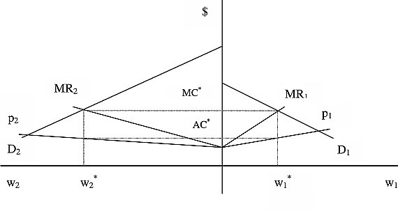
Figure 2
Illustration of variable unit pricing equilibrium.
[25] At the same time, the water utility will maximize net revenue for the given charge schedules:
satisfying the necessary conditions that the marginal charge for each consumer is equal to the marginal cost at equilibrium supply w*i, which is equal to equilibrium demand: By combining both consumer and water utility choice conditions (4)and (6), the necessary economic efficiency (EE) condition (2) will be satisfied.[26] Now we consider what parameter conditions will ensure that both efficiency and cost recovery are satisfied. For the linear unit price schedule pi(wi) = a + biwi with marginal charge MRi(wi) = a + 2biwi, the firm’s first‐order conditions require
At the supply‐demand equilibrium, the net benefit maximizing consumer will also set marginal benefit equal to the marginal charge: From (7), the equilibrium condition is that the demand charges are the same for each consumer relative to a reference consumer m:
2.3. Cost Recovery With Variable Unit Pricing
[27] For cost recovery (zero economic profit), total revenue equals joint cost:
Substituting from (9) for each consumer’s demand charge relative to consumer m: From (11), by factoring out the unit price for consumer m and dividing both sides of (11) by total water supply Σiw*i, the equilibrium unit price p* = a + bmw*m will equal average cost: Equation (9) implies the same unit price for all consumers at the equilibrium.[28] Figure 2 illustrates the VUP equilibrium with two consumers. The demand curve (Di) for each consumer is shown in one quadrant; it is the same as the marginal benefit schedule. At the equilibrium, each consumer’s demand curve intersects the marginal charge schedule (MRi) at the equilibrium demand w*i; at this demand, the marginal charge is equal to the equilibrium marginal cost MC*. The equilibrium unit price is found from where the equilibrium demand intersects the unit price schedule (pi); by construction, the unit price at equilibrium is equal to AC*. Also by construction, joint cost is equal to AC* times the sum of the two equilibrium demands. (Here with an increasing marginal charge, MC* exceeds AC*.) The consumer surplus (net benefit) for each consumer is indicated by the area above the average cost line and below the demand curve. The pricing equilibrium maximizes total consumer surplus (i.e., net benefits) over all consumers.
2.4. Variable Unit Pricing Parameter Determination
[29] Pricing parameters are determined simultaneously to satisfy economic efficiency and cost recovery at an equilibrium. Parameters result from simultaneously solving (7) and (12):
From (9), thus, a larger consumption will imply a smaller slope.[30] Equations (13) and (14) indicate that pricing parameters depend on the relative sizes of marginal cost and average cost as well as on the consumption level. The VUP schedule is increasing when the marginal cost curve is above the average cost curve, and decreasing in the reverse case.
2.5. Fairness Properties
[31] From (9), demands are proportional to total demand, with proportion inverse to the slope:
At equilibrium, the relative shares of revenue are equal to consumption shares: Since total revenues are constructed to be equal to total costs, by (16) each consumer’s charge at equilibrium is a proportion of total cost, with the proportion equal to the water consumption share. Proportional cost sharing is a common fairness property [Young and Peyton, 1995].
2.6. Comparison of Variable Unit Pricing to an Increasing Block Rate
[32] Figure 3 compares an increasing block rate schedule to the VUP equilibrium in Figure 2. The indicated IBR has three blocks for each consumer, respectively set at below AC*, at AC*, and at MC*, where AC* and MC* are at the same levels as in Figure 2. Since VUP maximizes total net benefit with cost recovery, any other pricing scheme, such as the indicated IBR, must either not cover cost or else have a lower total net benefit.

Figure 3
Comparison of increasing block rate to variable unit pricing.
[33] Consumer surplus (net gain) for the indicated IBR compared to the VUP equilibrium is illustrated in Figure 3. For both consumers, there is a small gain with IBR for the first block, because the price is less than AC*. For consumer 1, consumption occurs at the intersection of marginal benefit with the second block; consumption in block two is w1d, greater than the optimal w*1. The extra charge for the excess consumption by consumer 1 is offset by the extra benefit of the additional consumption. Consumer 2 has consumption in the third block w2d = w*2; there is a loss from IBR at this consumption because the price is higher, MC* instead of at AC*, which offset the gains in the first block from a lower charge. The consumer surplus gain by consumer 1 from the indicated IBR comes with a much larger loss for consumer 2.
[34] Cost recovery can also be examined in Figure 3. For consumer 2 in block three, the excess revenue over cost for the indicated IBR more than offsets the revenue loss in block one. For consumer 1, since there is increasing average cost, the excessive consumption in the second block is not supported by the revenue received, so that costs are not recovered for consumer 1. It is unlikely that total revenue equals cost for IBR, since cost recovery is not built into IBR as it is in VUP. IBR may produce either a loss or an excess in terms of cost recovery.
3. Variable Unit Pricing for a Supply Limit
[35] This section applies the pricing paradigm for a efficiency and cost recovery with a supply limit. Pricing parameters are now based on satisfying cost recovery with net benefit maximization, now subject to a supply constraint.
3.1. Economic Efficiency
[36] Given a limit L on the maximum amount of water that should be taken, economic efficiency is maximization of total net benefits subject to this supply limit:
The first‐order conditions for economic efficiency now include a shadow price μ from the resource constraint; the shadow price is the long‐term marginal cost to increase supply from the limit. The first‐order necessary conditions are: the marginal benefit for each water consumer should be equal to marginal cost plus the “shadow price” where the superscript L denotes evaluation at the constrained optimum:
3.2. Supply Demand Equilibrium With Variable Unit Pricing
[37] To satisfy constrained economic efficiency, the net revenue‐maximizing water utility should have the supply constraint added to its decision rules:
Denote the shadow price for the supply constraint by μ. An equilibrium allocation wiL with should satisfy marginal charge equal to marginal cost plus shadow price: The consumer problem is the same as in (3) above. Necessary conditions for the consumer are Efficiency with the supply constraint is satisfied by the combination of (20) and (21).[38] With variable unit pricing, from (20) the marginal charge should be equal to marginal cost plus the shadow price at a supply demand equilibrium:
Again, the equilibrium condition is that the demand charges are equal over consumers relative to a reference consumer m:
3.3. Cost Recovery
[39] Substituting (23), the cost recovery requirement with a supply limit becomes
Factoring out unit price, the equilibrium unit price is equal to average cost, here evaluated at the supply limit L: pL = C(L)/L.
3.4. Parameter Determination
[40] Parameters now include an additional parameter to be determined: the shadow price μ. Solving for slope and intercept from (22) and (24):
Increasing unit price schedules are again obtained when average cost is increasing. But if  is positive (i.e., the supply constraint is binding) and sufficiently large, increasing unit price schedules can be obtained even when average cost is decreasing.[41] From (25), we get the closed form for constrained consumption:
Summing over consumption, Solving for the shadow price μ from (26), the shadow price satisfies[42] Figure 4 illustrates the constrained supply demand equilibrium for variable unit pricing. The top half of the diagram is similar to Figure 2, except the demands and costs are at the constrained levels. The supply constraint is shown in the bottom‐right quadrant. The constrained equilibrium demands wiL occur at the intersection of the marginal charge with MC(L) + μ.
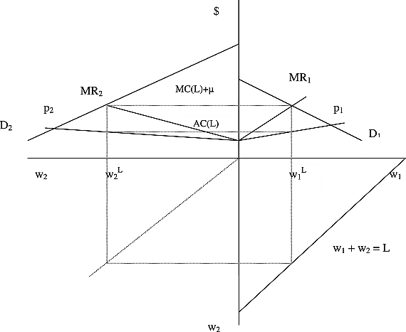
Figure 4
Illustration of variable unit pricing equilibrium with a supply constraint.
3.5. Fairness Properties
[43] From (26), water demands are in proportion to total supply L, inversely to slope:
Again, sharing of cost in proportion to consumption holds at the equilibrium: because total revenue is equal to supply cost.
4. Seasonal Pricing to Meet a Summer Capacity Limit
[44] In some geographic areas, reservoir storage capacity puts a limit on summer demands but not on winter demands. VUP with separate winter and summer rates can help satisfy the summer capacity limit, while covering costs over both seasons. The pricing method for this purpose is outlined and demonstrated below.
4.1. Economic Efficiency
[45] Winter demand is indicated by tɛW and summer demand by tɛS. Water use is differentiated by I and O for indoor and outdoor uses; wIt denotes indoor water use in a month of season t, and wOt denotes outdoor use in month t. To simplify the derivation, consumption can assumed to be the same in each month of a given season.
[46] Benefit functions for indoor and outdoor uses are assumed to be separable. Winter indoor demand and summer indoor demand are related because the same indoor technologies (shower, toilet, etc.) are used in both seasons. To simplify, the same benefit function can be assumed for indoor use for summer and winter. Further simplifying, summer and winter indoor use can be assumed to be the same. Outdoor demand is taken to be independent of indoor demand.
[47] To help distinguish between summer and winter costs, joint costs can be decomposed. Utility costs include both “operating and maintenance” (OM) and capital costs for long‐term facilities such as reservoirs. OM includes variable costs and fixed costs for billing and maintenance of facilities. Both components of OM can be apportioned by volume.
[48] Capital expenditure is discontinuous over years, depending on whether or not capital improvements are made in any given year. Payments to bond funds “smooth” capital expenditure over time. Below, K denotes reservoir capacity which constrains summer demand, and C(K) denotes annual revenue requirements for bond funds that finance capital costs.
[49] For economic efficiency, total net benefits should be maximized by water consumption for indoor and outdoor uses for both seasons, subject to the summer capacity constraint:
where Bi denotes benefit for consumer i for indoor or outdoor uses as noted. With the above simplifying assumptions, first‐order necessary conditions for efficient allocation are The right hand sides of the above equations represent total marginal cost, respectively for indoor and outdoor use. Because indoor use affects cost in both seasons, the marginal cost for winter indoor use includes the marginal OM effects of winter indoor use and summer indoor use plus the marginal capital cost. The marginal cost for summer outdoor use is marginal OM cost plus marginal capital cost.
4.2. Supply Demand Equilibrium With Variable Unit Pricing
[50] To simplify, rates can be set to be the same for each month of a given season (winter or summer). Monthly VUP charge schedules for consumers are specified separately by season:
where wit denotes total monthly water consumption by consumer i for a month in winter W or summer S; both indoor and outdoor uses are included in total water consumption for summer. Note that both slopes and intercept differ over seasons.[51] In winter months, the consumer chooses demand for monthly indoor use wiI to maximize net benefit, thus setting marginal benefit of indoor use equal to the marginal charge:
Denote the monthly indoor demand by  iI. Since winter and summer indoor use are assumed to be the same, only the outdoor decision is made in summer. Given monthly indoor use, the consumer chooses monthly outdoor demand to maximize net benefit; outdoor demand satisfies[52] The water utility should maximize net revenue over both seasons subject to the capacity constraint. Therefore, at equilibrium the marginal charge for each season is equal to both marginal benefit and marginal cost for that season. Again, equilibrium conditions are that demand charges are the same for each consumer relative to consumer m:
4.3. Cost Recovery and Pricing Parameters
[53] For cost recovery with seasonal pricing, equilibrium unit prices are assumed to be the same for summer and winter, and furthermore, equilibrium unit prices are set equal to average cost. In this way, total costs over summer and winter are covered by equilibrium unit prices.
[54] Parameters for each season can then be determined to simultaneously satisfy efficiency and cost recovery: Winter efficiency:
Summer efficiency: Winter cost recovery: Summer cost recovery: Solving (35) and (37) for winter parameters, and (36) and (38) for summer parameters: Winter:
Summer:
5. Empirical Applications
[55] Full information implementation of any pricing method requires both cost and demand data. For example, Barkatullah [1999] estimated both demand and cost functions to develop marginal cost pricing for India. Although methods for demand and cost estimation are found in many empirical studies, most studies report on either demand or cost estimation. Demand studies have been performed in many regions over the years, and there is wide variation in elasticity estimates, depending on the estimation method and geography. Demand studies have mostly been limited to households [e.g., Whitcomb et al., 1993].
[56] Cost function estimation is often based on cross‐sectional data [e.g., Renzetti, 2001; Sauer, 2005] and used for purposes of determining economies of scale in treatment and piping costs, or for measuring relative cost shares for labor and capital. Long‐run cost functions needed to address long‐run efficiency concerns are rarely available.
[57] For the Jordan example below, a “full information” approach is used. A long‐run cost function for raw water supply is first estimated on the basis of projected capacity expansion costs. Demand functions are also estimated on the basis of published elasticities. A mathematical programming method for constrained optimization is then applied to compute parameters relative to potential supply limits; see Appendix B for the solution method. The shadow price is obtained from the constrained optimization.
[58] As an alternative information treatment, “iterative pricing” can ease information needs. For this approach, data from a previous year are used to compute parameters. Enough iterations could in theory produce the full information solution but would in actuality be imperfect, because costs and demands would change as external conditions change. Still, pricing formulas based on theory can provide an objective way to determine rates.
[59] The Boulder example uses a previous year’s data on cost and demand to estimate pricing parameters for the succeeding year. Correspondingly, the computational method for pricing parameters is relatively simple: “spread sheets” are based on the seasonal pricing formulas.
5.1. Example for Amman, Jordan: “Full Information” Pricing and Cost Estimation
[60] As reported by World Bank [1997], public water supplied for Amman was about 90 million cubic meters (mcm). The current pricing method is increasing block rates, with an average price of 0.47 jd/cm (1 Jordanian dinar (jd) = U.S. $1.428) in 1997. Water in Amman has been rationed, resulting in privately trucked provision of water at rates as high as 1–2 jd/cm. Various projects have been proposed to expand the water supply.
5.1.1. Long‐Run Cost Function for Amman, Jordan
[61] A long‐run cost function to expand capacity was constructed from data on total construction costs for potential water supply projects [World Bank, 1997]. In Table 2, the “extra” cost for each project to increase supply is denoted by Δc; the “extra” volume from each project is denoted by Δw; the ratio Δc/Δw denotes the “extra” (marginal) construction cost per unit extra volume. “Economic cost” is the minimum cost to provide a given volume. Therefore, to minimize cost to produce any volume, projects should be adopted in order of increasing Δc/Δw. For example, the least cost to produce 25 million cubic meters (mcm) in Table 2 is to do the first two projects. The third and fourth projects would also give 25 mcm but at a greater cost.
Table 2. Long‐Run Construction Cost for Ordered Water Projects in Amman, Jordan
a
| Project |
Δw |
Δc |
Δc/Δw |
Volume ΣΔw |
Cost ΣΔc |
Average Cost Cost/w |
| Jafar/Shedia |
18 |
6 |
0.33 |
18 |
6 |
0.33 |
| Feedan Dam |
10 |
4 |
0.4 |
28 |
10 |
0.357 |
| Adasiyah Weir |
20 |
11 |
0.55 |
48 |
21 |
0.437 |
| Lagoon Wells |
5 |
5 |
1 |
53 |
26 |
0.490 |
| Wadi El Arab |
20 |
26 |
1.3 |
73 |
52 |
0.712 |
| Mujib Dam |
35 |
52 |
1.49 |
108 |
104 |
0.962 |
| Desalinization of urban Jordan |
60 |
100 |
1.66 |
168 |
204 |
1.21 |
| Aqaba desalinization |
20 |
40 |
2 |
188 |
244 |
1.30 |
| Wala Dam |
9.3 |
22 |
2.36 |
197.3 |
266 |
1.35 |
| Tannur Dam |
8.7 |
21 |
2.41 |
206 |
287 |
1.39 |
| Desalinization of Jordan |
5 |
14 |
2.80 |
211 |
301 |
1.43 |
| Disi‐Amman |
120 |
420 |
3.50 |
331 |
721 |
2.17 |
| Yarmouk River Dam |
85 |
303 |
3.56 |
416 |
1024 |
2.46 |
| Mujid Weir |
23 |
104 |
4.52 |
439 |
1128 |
2.5 |
[62] With a Cobb‐Douglas production function and cost minimization, the form of the cost function should depend on input prices (labor and capital) and volume. However, for this cross‐sectional study within the same time period, labor and capital prices are virtually the same over the study area. Since no identification of input price effects is needed, the construction cost function is specified only in terms of volume. The logarithmic form is
with a representing the effect of input prices and b representing the effect of production technology. The marginal cost function is MC(w) = b[C(w)]/w = b[AC(w)], where AC(w) represents the average cost function. Therefore, if b is greater than one, marginal expansion cost exceeds average expansion cost, implying rising average expansion cost. Regression analysis on data in Table 2 resulted in the following estimated long‐term expansion cost function (million Jordanian dinars (mjd) per mcm): with R2 = 0 0.9967. Because b exceeds 1, marginal and average costs are increasing. (The standard error of the slope coefficient is 0.028; the cost elasticity coefficient is in a confidence interval of two standard deviations about 1.7 with 0.97 probability.)[63] The current annual supply of raw water is taken to be 90 mcm plus 17 mcm transferred from agriculture at a low cost of 0.85 mjd (equal to 0.045 jd/cm times 17 mcm). Any raw water supply must, of course, be treated and piped. The current average water price (0.47 jd/cm) is assumed to be the average cost for piping and treating raw water, given sufficient capacity for piping and treating. The total annual cost (NC) for water supply, 107 mcm plus any new water w, is represented as the treatment cost for the existing and new raw water plus the annualized cost per unit of expansion:
where C(w) denotes the estimated long‐run cost function for construction. Construction cost is converted to an annual payment by dividing by 22.39, representing a 2% interest rate for a 30 year life of project. (Other interest rates and project life can be incorporated simply by changing this adjustment factor.) The marginal cost function is the derivative of (43).
5.1.3. Pricing Results
[65] Table 3 shows pricing parameters and shadow prices that correspond to varying supply limits and the unconstrained solution. Parameters were determined by nonlinear optimization for the specified cost and demand functions (see Appendix B). Because projects are discrete, but a continuous cost function is used to determine pricing, costs are not exactly covered by the indicated prices; adjustments could be added as a lump sum charge.
Table 3. Variable Unit Pricing With a Supply Constraint, Amman, Jordan
|
Supply Constraint |
| Unconstrained |
151 mcm |
131 mcm |
| Charge intercept a (jd/cm) |
0.453393 |
0.319213 |
0.127540 |
| Charge slope (jd/mcm) |
|
|
|
| Household |
306.5 |
1811.5 |
4570.0 |
| Commercial |
455.4 |
2633.2 |
6476.2 |
| Equilibrium unit price (jd/cm) |
0.484691 |
0.481272 |
0.478535 |
| Shadow price (jd/cm) |
0 |
0.138063 |
0.336766 |
| Demand (mcm) |
171.8 |
151 |
131 |
| Household |
102.1 |
89.4 |
76.8 |
| Commercial |
68.7 |
61.5 |
54.1 |
| Total charge (mjd) |
82.7 |
72.6 |
62.6 |
| Household |
49.4 |
43.0 |
36.7 |
| Commercial |
33.3 |
29.6 |
25.8 |
[66] Supply limit levels were chosen arbitrarily for demonstration purposes. Meeting the demand of 171 mcm (unconstrained solution) with the available supply of 107 would require additional 64 mcm; correspondingly, the first five projects (up to and including Wadi El Arab) should be built. For a supply limit of 151 mcm, the additional 44 mcm could be supplied by three projects, up to and including Adasiyah Weir. For the more restrictive limit of 131 mcm, only two projects (up to and including Feedan Dam) would be needed.
[67] As the supply limit becomes more restrictive, the unit price parameters in Table 3 exhibit increasing slope and decreasing intercept. The resulting equilibrium unit price decreases as the supply limit becomes more restrictive. Because cost is less for a smaller supply, and revenues must cover a smaller cost, setting supply limits with VUP pricing can result in reduced supply costs and reduced water bills.
5.2. Example of Seasonal Pricing: Boulder, Colorado (2001)
[68] The following example demonstrates the less data intensive approach of iterative pricing. Two steps for a past year’s water data were required: (1) developing consumption data for a representative typology of water consumers through detailed utility records and (2) estimating marginal and average costs by season. Then, slopes and intercept and corresponding rate schedules were computed by consumer type. (Computations used a spreadsheet. Consumer type details and spreadsheets for Boulder, Colorado, are available from the author.)
5.2.1. Estimating Marginal and Average Costs
[69] Operating and maintenance (OM) and capital data were available only in annual terms from Boulder utility auditing documents. Average OM and capital costs were obtained by dividing total costs by total annual consumption.
[70] Marginal OM and marginal capital costs had to be estimated by season. Marginal OM cost and marginal capital cost vary by season because of the summer capacity constraint. Marginal capital cost is taken to be zero in the winter, because there is excess capacity. For winter, marginal OM cost is taken to be equal to average treatment and power cost, since only treatment and power expansion is needed to increase volume in winter.
[71] In summer, raw water must be obtained from alternative sources when capacity is exceeded. A reservoir at Windy Gap provides peaking supply for Boulder. In Boulder rate publications, the last block of the IBR schedule has been described to be the summer marginal cost to obtain peaking supply. For 2001, the last block rate was $3.85 per 1000 gal. (1 gal. = 3.785 L).The breakdown for 1992 (the most recent cost breakdown) was 46% for variable cost and 54% for capital cost. These proportions were applied to the 2001 total marginal cost to obtain the indicated summer marginal cost breakdowns for OM and capital.
[72] Table 4 shows the resulting cost estimates. For both OM and capital, average cost exceeds marginal cost in winter, whereas marginal cost exceeds average cost in summer. Therefore unit pricing will have a negative slope for winter, whereas summer pricing will have a positive slope.
Table 4. Boulder Cost Breakdown for 2001
a
|
Annual |
Winter |
Summer |
| OM cost |
$8,288,607 |
|
|
| Capital cost |
$7,852,781 |
|
|
| Total average cost/1000 gal |
$2.479 |
|
|
| OM average cost/1000 gal. |
|
$1.273 |
$1.273 |
| Capital average cost/1000 gal. |
|
$1.206 |
$1.206 |
| OM marginal cost/1000 gal. |
|
$0.260 |
$1.770 |
| Capital marginal cost/1000 gal. |
|
$0.000 |
$2.070 |
5.2.2. Demand by Water Consumer Types
[73] Boulder Utilities Division develops rates for types of water consumers rates: single family residence, trailer parks, multifamily residences, commercial/industrial, and sprinklers. (Separate rates are given “inside” and “outside” the city for cost reasons.) To provide more finely tuned rates, here consumer types were further subdivided into “low,” “medium,” and “high” types, for a total of fifteen types, where “medium” represents the typical consumer for each type. The distribution of use by types was constructed to match 2001 consumption data.
5.2.3. Seasonal Pricing for Boulder
[74] Tables 5 and 6 show VUP rate schedules for two of the fifteen consumer types for winter and summer, respectively: the average single family residence and the average commercial account inside the city limits. By construction, the unit price each season for average use for each type is equal to average cost (here $2.48). In Tables 5 and 6, average cost and average quantity for each type are indicated by bold font. Those who use more than the average will pay a unit charge higher than average cost, and conversely for those who use less than average.
Table 5. Variable Unit Pricing Schedule for Average Boulder Household for the 2001 Simulation
a
|
Unit Price |
Total Bill |
| Winterb |
| 1 |
$2.82 |
$2.82 |
| 2 |
$2.74 |
$5.47 |
| 3 |
$2.65 |
$7.95 |
| 4 |
$2.56 |
$10.26 |
| 5 |
$2.48 |
$12.39 |
| 6 |
$2.39 |
$14.36 |
| 7 |
$2.31 |
$16.15 |
| 8 |
$2.22 |
$17.77 |
| 9 |
$2.14 |
$19.22 |
|
| Summerc |
| 9 |
$2.34 |
$21.09 |
| 10 |
$2.48 |
$24.79 |
| 11 |
$2.62 |
$28.77 |
| 12 |
$2.75 |
$33.01 |
| 13 |
$2.89 |
$37.53 |
| 14 |
$3.02 |
$42.33 |
| 15 |
$3.16 |
$47.39 |
| 16 |
$3.29 |
$52.73 |
| 23 |
$4.25 |
$97.71 |
Table 6. Variable Unit Pricing Schedule for Average Boulder Commercial Account for the 2001 Simulation
a
|
Unit Price |
Total Bill |
| Winterb |
| 79 |
$2.50 |
$197.47 |
| 80 |
$2.49 |
$199.56 |
| 81 |
$2.49 |
$201.63 |
| 82 |
$2.48 |
$203.70 |
| 83 |
$2.48 |
$205.75 |
| 84 |
$2.47 |
$207.80 |
| 85 |
$2.47 |
$209.83 |
| 86 |
$2.46 |
$211.86 |
|
| Summerc |
| 127 |
$2.42 |
$307.03 |
| 128 |
$2.43 |
$310.76 |
| 129 |
$2.44 |
$314.50 |
| 130 |
$2.45 |
$318.27 |
| 131 |
$2.46 |
$322.06 |
| 132 |
$2.47 |
$325.87 |
| 133 |
$2.48 |
$329.70 |
| 134 |
$2.49 |
$333.55 |
[75] For both indicated consumer types, the base charge is the predominant charge. The total bill is a result of both base and demand charges. The small negative slope for winter is offset by the much larger base charge, so that the total charge for winter increases approximately linearly with water use. The summer rate reflects a positive demand charge; the total charge increases quadratically with use.
[76] The average Boulder household uses about 5000 gallons per month in winter, and the summer use is about double the winter use. In spite of different slopes and intercepts, the result is approximately linear: the typical household monthly bill for summer is about twice that for winter for about twice as much consumption. The typical commercial account uses 83,000 gallons in the winter and 133,000 gallons in the summer. VUP results in a 60% increase in the average commercial summer bill over the winter bill for about a 60% consumption increase. Even thought the total bill is quadratic in volume, near linearity between volume and use is due to the predominance of the base charge over the demand charge. Still, the demand charge does not have to be very large to have an incentive effect on demand.
[77] Comparing rates by use types, the commercial rate has a flatter slope than the household because of higher water use by the commercial consumer (the use level determines the denominator for the slope). Still, the total charge for the household is much less than for the commercial consumer because of the commercial consumer’s much higher volume.
[78] Using the iterative method, costs for a given year may not be exactly covered by parameters based on data from a previous year; there may be an excess or insufficiency, depending on use and cost trends. Adjustments to cover cost can be made in a future year.
[79] Table 7 compares VUP and IBR rates for a typical Boulder household with monthly consumption as indicated by season. VUP bills for all months are higher than for IBR, but IBR rates for 2001 did not cover costs and were raised in 2004. Interestingly, the summer maximum charge is about eight times the predominant winter charge for both rate structures.
Table 7. Monthly Bill Comparisons for a Typical Boulder Household: 2001 VUP and 2001 IBR
| Monthly Use (gal.) |
Seasona |
VUP Monthly Bill |
IBR Consumption by Block (gal.) |
IBR Monthly Bill |
| $1.50 |
$2.55 |
$3.85 |
| 5 × 10³ |
W |
$12.39 |
5 × 10³ |
|
|
$7.50 |
| 5 × 10³ |
W |
$12.39 |
5 × 10³ |
|
|
$7.50 |
| 5 × 10³ |
W |
$12.39 |
5 × 10³ |
|
|
$7.50 |
| 6 × 10³ |
W |
$14.36 |
5 × 10³ |
1 × 10³ |
|
$10.05 |
| 8 × 10³ |
W |
$17.77 |
5 × 10³ |
3 × 10³ |
|
$15.15 |
| 15 × 103 |
S |
$47.39 |
5 × 10³ |
10 × 103 |
|
$33.00 |
| 23 × 103 |
S |
$97.71 |
5 × 10³ |
13 × 103 |
5 × 10³ |
$59.50 |
| 17 × 103 |
S |
$58.34 |
5 × 10³ |
12 × 103 |
|
$38.10 |
| 16 × 103 |
S |
$52.73 |
5 × 10³ |
11 × 103 |
|
$35.55 |
| 10 × 103 |
S |
$24.79 |
5 × 10³ |
5 × 10³ |
|
$20.25 |
| 5 × 10³ |
S |
$8.99 |
5 × 10³ |
|
|
$7.50 |
| 5 × 10³ |
W |
$12.39 |
5 × 10³ |
|
|
$7.50 |
| Year total |
|
$371.64 |
|
|
|
$249.50 |
5.2.4. Summary of Boulder Rate History
[80] The Boulder experience with the process of making rate changes demonstrates the complexity and transactions costs of rate setting. Starting in 2004, public hearings were held with much public discussion. Citizen participation in rate hearings indicated that water consumers are interested in their rate structures and willing to be involved in water pricing decisions. Much of the public discussion of rate structures had to do with fairness.
[81] In January 2007, the method of rate making was changed from IBR to a “water budget” approach. For the water budget for households, the utility specifies a target for water use on the basis of a household’s lot size; aerial photographs for 2003 are used for the household budget assessment. The budget for outdoor use is based on horticultural research regarding the amount of water necessary for healthy bluegrass lawns in Colorado; the budget can vary monthly on the basis of watering needs. Indoor needs are based on 7000 gallons for a family of four. If dissatisfied with their budgets, households can appeal to the utility. For commercial/industrial users, the monthly water budget is based on 2005 actual average monthly use. (See Basics of your water budget, www.bouldercolorado.gov)
[82] For drought situations, the water budget provides an alternative to unpopular restrictions used in the past. To address droughts such as occurred in 2002, the stated goal of the water budget is for the utility to be able to adjust rates rapidly. When droughts occur, water budget levels can be changed while maintaining the structure of rate blocks.
[83] The same block structure is used for all user types while varying their allotted water budgets. Five rate blocks are assigned in relationship to the water budget: the first block rate holds for up to 60% of the allotted water budget, the second block is 61% to 100%, the third block is 101% to 150%, the fourth block is 151% to 200%, and the last block is for volumes greater than 200%; the same structure is used year round (summer use typically falls into the fourth or fifth blocks). Rates are set by block: Block 2, the “base rate, is set at $2.50 per 1000 gals., Block 4 is three times the base rate, and Block 5 is five times the base rate. The Boulder water utility reports that 2007 rates achieve nearly proportionate sharing of costs by volume of consumer type. (See Updated water revenue and use totals, January through December 2007, http://ci.boulder.co.us).
[84] The water budget method is still a form of IBR in that blocks require parameterization for price levels and percentages of water budget. The same shortcomings of IBR hold for the water budget: it does not guarantee that supply costs will be exactly covered or that a target supply level will be met. A Boulder conservation group cautions: “Reductions in water consumption and the new rate increase plan can create infrastructure budget deficits long term but in the short run it should create windfall revenue increases until conservation takes hold. What is Boulder going to do with these collection windfalls?…” (http://www.boulderflycasters.org/reelnews/2007/feb/index.htm).
6. Contexts for Variable Unit Pricing
[85] For a municipal utility, VUP pricing rules can be used directly by the government agency that supplies water. For a contractual arrangement with a private supplier, pricing rules could be defined as part of the arrangement. However, since the unit pricing formulas result in zero profit, an additional management fee would be required for a private utility to operate. Specifying the pricing rule for a private utility is similar to a regulatory agency setting rules such as an allowed rate of return or a pricing cap. (Loehman [2004] discussed the economic organization implications of variable unit pricing in more detail.)
[86] An important context for variable unit pricing is planning for integrated water resource management (IWRM) and water demand management (WDM). Water demand management refers to conservation on the demand side as an alternative to more costly supply expansion. IWRM refers to a participatory planning process to determine how best to meet society’s long‐term water needs while maintaining essential ecological services (What is integrated water resources Management?, http://www.usaid.gov/, 2006). Drought planning is another context in which communities develop conservation and management plans and rules for low water supply.
[87] In response to prolonged drought with reduced supply or to reduce excessive groundwater pumping, a supply limit could be set as an alternative to seeking costly new supplies. Then, variable unit pricing would help to ensure that costs would be covered while providing incentives for meeting the supply limit. Because VUP is formula driven in terms of cost and capacity/limits, alternative scenarios could be readily translated by planners into pricing implications.
[88] One principle of IWRM is public involvement. Deliberation is more specific: reasoned discussion among citizens that leads to an agreement that is acceptable to all. Deliberation is being applied to the management of water utilities; see the examples of Flynn and Boudouris [2005] and the Municipal Plan of the Township of Centre Wellington in Ontario Canada (www.beyondapipedream.com). Deliberation among citizens served by a water utility can help to make socially acceptable decisions about capacity expansion versus setting limits. By comparing alternative costs, supply levels, and pricing implications, citizens could determine whether they would be willing to pay more to increase supply, or to pay less while facing supply limits.
7. Conclusions
[89] Variable unit pricing provides an objective foundation for water utility pricing, with well‐defined formulas to specify rate making. Furthermore, it is designed to satisfy, in theory, the desirable properties of cost recovery and economic efficiency. Total bills based on unit pricing may also be easier for consumers to comprehend than increasing block rates.
[90] This paper showed applications of variable unit pricing to situations not addressed by increasing block rates: meeting supply limits and seasonal capacity constraints. Two case studies showed the efficacy of VUP for supply limits and seasonal pricing while drawing on two different empirical methods. The Jordan study used “full information” to show that pricing for a supply limit can help avoid more costly system expansion. The Boulder study used “iterative information,” employing seasonal pricing with separate unit price schedules for winter and summer on the basis of differences between average and marginal costs for these seasons. The resulting increased demand charges for summer, to provide incentives to reduce summer use, may be preferred by consumers to unpopular use restrictions.
Acknowledgments
[99] Thanks to Bronwyn Weygandt, Director of Billing, Boulder Water, for consumption and billing data. Thanks to Carol Linn, Financial Officer of Boulder Water, for cost data. Charles Howe, Department of Environment and Society, Institute for Behavioral Science, University of Colorado, is thanked for providing much encouragement during the course of this work and for pointing attention to pricing by consumer type. Keith Willett, Department of Economics, Oklahoma State University, is thanked for very helpful review comments. George Tolley, Economics, University of Chicago, is thanked for encouraging me to develop interpretations and applications.
Appendix A:: Parameter Determination by Water Consumer Type
[91] The derivation of pricing parameters above was for individualized rate structures for each consumer, intractable especially for larger water supply systems because of information, computation, and administrative needs. It is reasonable to seek to simplify rate structures by grouping water consumers by type such that consumers of the same type will receive the same price schedule.
[92] Below, a method to structure unit pricing by type of consumer is suggested. The method of pricing by group has less tidy properties than individualized rate structures as described above, because costs may not be exactly covered and efficiency is not perfectly achieved. Still, the method has a theoretical foundation and reasonable properties.
[93] Suppose water consumers can be grouped, with groups denoted by k and an individual member of a group denoted by ik. Each group has an average use level
where nk denotes the number of members in group k. There is a distribution of individual demands about the group average:[94] For group charge schedules, we seek to define a slope bk for each group with a common intercept. A natural extension of the individual slope and intercept parameter formulas is to solve the following simultaneous system for group parameters:
That is, the average use for each group would be charged a unit price equal to average cost, and the marginal charge for the average use would be set at marginal cost.[95] Unfortunately, there is an imperfection from pricing by consumer type. Given charge schedules by type, suppose water consumers would maximize their net benefits. The corresponding first‐order condition are that marginal benefit should equal the marginal charge for each consumer:
If at the same time, the water utility satisfies (A3), the efficiency conditions – marginal benefit by individual consumer equals marginal cost – are only approximately satisfied.[96] To justify (A2) and (A3), consider the utility’s expected net revenue. Denote variance of the error by group by σk2; the sum of the squared error in (A1) is equal to nkσk2. Substituting (A1) in the revenue expression and taking expectations, total expected net revenue E(NR) is equal to:
given zero means of the error terms in (A1) and independence of the error terms from average use levels. By maximizing expected net revenue (A5) over group average use, (A3) will be satisfied by the utility. Furthermore, satisfying (A2) will result in positive expected net revenue at the utility optimum, i.e., cost recovery is more than achieved. To minimize excess revenue over cost, grouping should be defined to minimize Σnkσk2.
Appendix B:: Nonlinear Solution Method for Full Information
[97] To solve for the equilibrium with full information about cost and marginal benefits, a nonlinear solver such as GAMS (General Algebraic Modeling System, http://www.gams.com) can be used. A procedure for solving for parameters a, {bj}, {wj} is to solve the following system, which has equilibrium conditions as constraints:
The slack variables lj, kj, and τ should be zero for an exact solution to the equilibrium system.[98] Any other supply constraints – such as annual or seasonal limits – can also be added, and optimization of the system then allows determination of the corresponding shadow prices.
Supporting Information